European Windows 2019 Hosting BLOG

BLOG about Windows 2019 Hosting and SQL 2019 Hosting - Dedicated to European Windows Hosting Customer

European SQL Server 2022 Hosting :: SQL Server System-Versioned Temporal Tables

clock May 30, 2024 07:30 by author Peter

A potent SQL feature that makes it possible to store previous data changes alongside the current data is system-versioned temporal tables. This functionality is very helpful for data consistency, auditing, and tracking changes over time. This paper examines the background, development, and necessity of system-versioned temporal tables, as well as their limitations and the most recent developments in the field. Furthermore, an example SQL code is included to show how they should be implemented.

Evolution and History
The necessity of handling time-sensitive data in databases gave rise to the idea of temporal tables. At first, handling historical data required developing unique solutions with complicated queries, extra tables, and triggers. These methods were frequently laborious and prone to mistakes.

With the release of SQL:2011, an ISO standard for SQL that outlined the support for system-versioned tables, temporal tables became a native capability. Subsequently, this capability was incorporated into the systems of major database suppliers, such as Microsoft SQL Server, Oracle, IBM Db2, and PostgreSQL, which made handling historical data easier.

The Need for System-Versioned Temporal Tables
System-versioned temporal tables address several critical needs.

  • Auditing and Compliance: Many industries require a detailed audit trail for compliance with regulatory standards. Temporal tables provide a straightforward way to track and retrieve historical data changes.
  • Data Analysis: Analyzing data changes over time can provide valuable insights. Temporal tables make it easier to perform such time-based analyses without additional overhead.
  • Error Correction: In case of accidental data modifications or deletions, temporal tables allow for easy retrieval of previous states, facilitating quick error correction.
  • Consistency and Integrity: Temporal tables ensure data consistency and integrity by maintaining a history of changes automatically, reducing the risk of data loss or corruption.

Drawbacks
Despite their advantages, system-versioned temporal tables have some drawbacks.

  • Storage Overhead: Storing historical data can significantly increase storage requirements. Proper planning and management are necessary to handle this overhead.
  • Performance Impact: Maintaining history can impact write performance, especially in high-transaction environments. Optimizations and indexing strategies are needed to mitigate this.
  • Complexity: Understanding and managing temporal tables can add complexity to the database schema and queries, requiring additional learning and expertise.

Latest Version and Features
The latest advancements in system-versioned temporal tables focus on improving performance, scalability, and ease of use. For instance, SQL Server 2019 introduced enhancements such as in-memory OLTP support for temporal tables, which helps to mitigate performance impacts.

Moreover, modern implementations provide better tools for querying historical data, including enhanced support for time-based joins and advanced filtering options.

Sample SQL Code
Below is a sample SQL code to create and use a system-versioned temporal table in Microsoft SQL Server.
-- Create a table with system-versioning enabled
CREATE TABLE Employees
(
    EmployeeID INT PRIMARY KEY,
    Name NVARCHAR(100),
    Position NVARCHAR(100),
    Salary DECIMAL(10, 2),
    SysStartTime DATETIME2 GENERATED ALWAYS AS ROW START HIDDEN NOT NULL,
    SysEndTime DATETIME2 GENERATED ALWAYS AS ROW END HIDDEN NOT NULL,
    PERIOD FOR SYSTEM_TIME (SysStartTime, SysEndTime)
)
WITH
(
    SYSTEM_VERSIONING = ON (HISTORY_TABLE = dbo.EmployeesHistory)
);

-- Insert data
INSERT INTO Employees (EmployeeID, Name, Position, Salary)
VALUES (1, 'John Doe', 'Manager', 75000);

-- Update data
UPDATE Employees
SET Salary = 80000
WHERE EmployeeID = 1;

-- Query current data
SELECT * FROM Employees WHERE EmployeeID = 1;

-- Query historical data
SELECT * FROM EmployeesHistory WHERE EmployeeID = 1;

-- Query data at a specific point in time
SELECT * FROM Employees
FOR SYSTEM_TIME AS OF '2024-01-01T00:00:00.0000000'
WHERE EmployeeID = 1;


Conclusion
System-versioned temporal tables are a significant evolution in SQL databases, addressing the need for robust time-based data management. While they come with certain drawbacks, their benefits in terms of auditing, compliance, data analysis, and error correction make them invaluable in modern data management. Continuous advancements in this area promise even greater efficiency and usability, making temporal tables an essential tool for contemporary database solutions.

HostForLIFEASP.NET SQL Server 2022 Hosting


European SQL Server 2022 Hosting :: How SQL Server Processes Your Query?

clock May 28, 2024 09:32 by author Peter

The main relational database product from Microsoft, SQL Server, is a complicated piece of software with a straightforward purpose: to process SQL queries and produce results as soon as feasible. Gaining an understanding of SQL Server's low-level workings can significantly boost the effectiveness and performance of your database applications. The goal of this blog is to clarify the procedure SQL Server goes through when handling your queries.

Parsing and Normalization
First, when a SQL query arrives, it undergoes parsing and normalization.

  • Parsing: This phase involves scanning the incoming SQL text and dividing it into individual keywords, expressions, and identifiers. Invalid syntax would lead to query termination at this stage.
  • Normalization: This stage, also known as algebrization, converts parsed SQL query to a tree of logical operators termed as “query tree”.

Compilation
Next, SQL Server attempts to compile the query.

  • Optimization: SQL Server's Query Optimizer evaluates different plans to execute and chooses the least costly one. The process it uses, interestingly, isn't exhaustive — checking every possible plan would require an unrealistic amount of time for complex queries. Instead, the optimizer uses heuristic algorithms and statistical metadata from distribution statistics objects to create a reasonable plan quickly.
  • Plan Generation: After the query optimization, SQL Server generates the query execution plan - the blueprint to execute the given query. These plans are stored in the "Plan Cache". If similar queries are used often, SQL Server can save resources by caching and reusing their execution plans.

Execution
With the plan in place, SQL Server moves to executing the query.

  • Execution Context Generation: The Query Execution engine generates an execution context for the query, a set of instructions that execute in line with the generated plan.
  • Data Retrieval: The system then undertakes activities like opening file handles, memory allocation based on the generated steps. Pages with necessary records are loaded from the disk into the buffer, if they aren't already there.
  • Data Return: After all processing steps are carried out; the Server retrieves data according to the instructions and sends it back to the client who requested it.

Conclusion

SQL query processing is a complex process that involves several steps, from parsing to execution. SQL Server is tuned using strategies like cost-based query optimization and execution plan caching to manage this operation as fast and effectively as possible. When working with SQL Server in real-world applications, knowing the intricacies of this process can help tremendously with diagnostics and performance optimization.

Recall that a significant portion of SQL Server's performance is dependent on elements other than the query processing phase. These include the appropriate use of indexes, current statistics, proper database design, well-structured queries, suitable hardware, and routine maintenance. But the first step to becoming an expert with this potent relational database engine is to have a comprehensive grasp of the process that SQL Server goes through, from accepting a request to producing a response.

HostForLIFEASP.NET SQL Server 2022 Hosting


European SQL Server 2022 Hosting :: How to Work with LEAD and LAG Window Functions in SQL?

clock May 21, 2024 10:28 by author Peter

Numerous analytical functions in SQL enable us to carry out intricate computations and data analysis jobs. SQL window functions called LEAD and LAG let us access data from other rows that are part of the same resultant row. They are frequently utilized in conjunction with the OVER clause, which specifies how the result set is divided and arranged. The value for the LAG function comes from a row that comes before the current one, whereas the value for the LEAD function comes from a row that comes after the current one.

The offset parameter, which indicates how many rows to advance or retract from the current row, is accepted by both functions. Let's examine the syntax, usage cases, and examples of LEAD and LAG to better understand how they work.

LEAD and LAG Functions Syntax

--LAEAD Function Syntax:
LEAD(column_name, offset, default_value) OVER (
    PARTITION BY partition_expression
    ORDER BY order_expression
)

--LAG Function Syntax:
LAG(column_name, offset, default_value) OVER (
    PARTITION BY partition_expression
    ORDER BY order_expression
)
  • column_name: Name of the column from which you want to retrieve the value.
  • offset: Number of rows to move forward (LEAD Function) or backward (LAG Function) from the current row. The default value is 1 and should be positive.
  • default_value (optional): Default value to return if the lead or lag value is NULL or if there is no subsequent row within the partition.
  • PARTITION BY (optional): Divides the result set into partitions based on the specified expression.
  • ORDER BY: Specifies the ordering of rows within each partition.

Lets take an example for LEAD and LAG functions.create a table named sales with the following structure:

-- Create salas table
CREATE TABLE sales (
    product VARCHAR(50),
    year INT,
    sales_amount DECIMAL(10,2)
);

-- Add some dummy data into the table
INSERT INTO sales (product, year, sales_amount) VALUES
('Apples', 2021, 1500.50),
('Bananas', 2021, 2500.75),
('Carrots', 2021, 3200.00),
('Apples', 2022, 1700.30),
('Bananas', 2022, 2900.20),
('Carrots', 2022, 3400.60),
('Apples', 2023, 1800.00),
('Bananas', 2023, 3100.45),
('Carrots', 2023, 3600.80),
('Oranges', 2021, 1100.25),
('Oranges', 2022, 1300.50),
('Oranges', 2023, 1400.75),
('Tomatoes', 2021, 1200.00),
('Tomatoes', 2022, 1500.35),
('Tomatoes', 2023, 1600.90);

Retrieving the next product's sales amount using LEAD function

SELECT product,year,sales_amount,
    LEAD(sales_amount, 1, 0) OVER (
        ORDER BY year, product
    ) AS next_product_sales
FROM
    sales ;

--Sample O/P
+----------+------+---------------+--------------------+
| product  | year | sales_amount  | next_product_sales |
+----------+------+---------------+--------------------+
| Apples   | 2021 |        1500.5 |             2500.75 |
| Bananas  | 2021 |        2500.75|              3200.0 |
| Carrots  | 2021 |         3200.0|             1100.25 |
| Oranges  | 2021 |        1100.25|              1200.0 |
| Tomatoes | 2021 |         1200.0|              1700.3 |
| Apples   | 2022 |         1700.3|              2900.2 |
| Bananas  | 2022 |         2900.2|              3400.6 |
|.......    .....          .......               ......
+----------+------+---------------+--------------------+

In above Query , we use the LEAD function to retrieve the sales amount of the next product in the same year. If there is no subsequent product, the default_value of 0 is returned.

Retrieving the prev product's sales amount using LAG function

SELECT product, year,sales_amount,
    LAG(sales_amount, 1, 0) OVER (
        ORDER BY year, product
    ) AS prev_product_sales
FROM sales;

--Sample O/P

+----------+------+---------------+--------------------+
| product  | year | sales_amount  | next_product_sales |
+----------+------+---------------+--------------------+
| Apples   | 2021 |        1500.5 |                0.0 |
| Bananas  | 2021 |        2500.75|             1500.5 |
| Carrots  | 2021 |         3200.0|             2500.75|
| Oranges  | 2021 |        1100.25|              3200.0|
| Tomatoes | 2021 |         1200.0|             1100.25|
| Apples   | 2022 |         1700.3|              1200.0|
| .....      ....           .....             ......
+----------+------+---------------+--------------------+

In above Query , we use the LEAD function to retrieve the sales amount of the next product in the same year. If there is no subsequent product, the default_value of 0 is returned.

Use Case

Suppose we want to analyze the sales data for each product, not only by comparing the current year's sales with the previous year but also by looking forward to the next year's sales. We can achieve this by combining the LEAD and LAG functions in a single query.

SELECT product, year, sales_amount,
    sales_amount - LAG(sales_amount, 1) OVER (
        PARTITION BY product
        ORDER BY year
    ) AS year_over_year_diff,
    LEAD(sales_amount, 1, 0) OVER (PARTITION BY product
        ORDER BY year) - sales_amount AS next_year_diff
FROM sales ORDER BY product, year;

-- Sample O/P
+----------+------+---------------+------------------+----------------+
| product  | year | sales_amount  | year_over_year_diff | next_year_diff |
+----------+------+---------------+------------------+----------------+
| Apples   | 2021 |        1500.5 |              NULL |          199.8 |
| Apples   | 2022 |        1700.3 |             199.8 |           99.7 |
| Apples   | 2023 |         1800.0|              99.7 |        -1800.0 |
| Bananas  | 2021 |        2500.75|              NULL |          399.45|
| Bananas  | 2022 |        2900.2 |             399.45|          200.25|
| Bananas  | 2023 |        3100.45|             200.25|        -3100.45|
| Carrots  | 2021 |         3200.0|              NULL |          200.6 |
| .....      ...            ....              .....          ....... ...
+----------+------+---------------+------------------+----------------+

In the LAG Functions we are calculating the year-over-year difference in sales by subtracting the previous year's sales amount from the current year's sales amount. In the LEAD Functions we are calculating the difference between the next year's sales amount and the current year's sales amount. By including both expressions in the same query, we can analyze the sales data for each product by looking at the year-over-year difference as well as the projected difference for the next year.

HostForLIFEASP.NET SQL Server 2022 Hosting


European SQL Server 2022 Hosting :: How to Work with LEAD and LAG Window Functions in SQL?

clock May 21, 2024 09:48 by author Peter

Numerous analytical functions in SQL enable us to carry out intricate computations and data analysis jobs. SQL window functions called LEAD and LAG let us access data from other rows that are part of the same resultant row. They are frequently utilized in conjunction with the OVER clause, which specifies how the result set is divided and arranged. The value for the LAG function comes from a row that comes before the current one, whereas the value for the LEAD function comes from a row that comes after the current one.

The offset parameter, which indicates how many rows to advance or retract from the current row, is accepted by both functions. Let's examine the syntax, usage cases, and examples of LEAD and LAG to better understand how they work.

LEAD and LAG Functions Syntax
--LAEAD Function Syntax:
LEAD(column_name, offset, default_value) OVER (
    PARTITION BY partition_expression
    ORDER BY order_expression
)

--LAG Function Syntax:
LAG(column_name, offset, default_value) OVER (
    PARTITION BY partition_expression
    ORDER BY order_expression
)

  • column_name: Name of the column from which you want to retrieve the value.
  • offset: Number of rows to move forward (LEAD Function) or backward (LAG Function) from the current row. The default value is 1 and should be positive.
  • default_value (optional): Default value to return if the lead or lag value is NULL or if there is no subsequent row within the partition.
  • PARTITION BY (optional): Divides the result set into partitions based on the specified expression.
  • ORDER BY: Specifies the ordering of rows within each partition.


Lets take an example for LEAD and LAG functions.create a table named sales with the following structure:
-- Create salas table
CREATE TABLE sales (
    product VARCHAR(50),
    year INT,
    sales_amount DECIMAL(10,2)
);

-- Add some dummy data into the table
INSERT INTO sales (product, year, sales_amount) VALUES
('Apples', 2021, 1500.50),
('Bananas', 2021, 2500.75),
('Carrots', 2021, 3200.00),
('Apples', 2022, 1700.30),
('Bananas', 2022, 2900.20),
('Carrots', 2022, 3400.60),
('Apples', 2023, 1800.00),
('Bananas', 2023, 3100.45),
('Carrots', 2023, 3600.80),
('Oranges', 2021, 1100.25),
('Oranges', 2022, 1300.50),
('Oranges', 2023, 1400.75),
('Tomatoes', 2021, 1200.00),
('Tomatoes', 2022, 1500.35),
('Tomatoes', 2023, 1600.90);

Retrieving the next product's sales amount using LEAD function.

SELECT product,year,sales_amount,
    LEAD(sales_amount, 1, 0) OVER (
        ORDER BY year, product
    ) AS next_product_sales
FROM
    sales ;

--Sample O/P
+----------+------+---------------+--------------------+
| product  | year | sales_amount  | next_product_sales |
+----------+------+---------------+--------------------+
| Apples   | 2021 |        1500.5 |             2500.75 |
| Bananas  | 2021 |        2500.75|              3200.0 |
| Carrots  | 2021 |         3200.0|             1100.25 |
| Oranges  | 2021 |        1100.25|              1200.0 |
| Tomatoes | 2021 |         1200.0|              1700.3 |
| Apples   | 2022 |         1700.3|              2900.2 |
| Bananas  | 2022 |         2900.2|              3400.6 |
|.......    .....          .......               ......
+----------+------+---------------+--------------------+

In above Query , we use the LEAD function to retrieve the sales amount of the next product in the same year. If there is no subsequent product, the default_value of 0 is returned.

Retrieving the prev product's sales amount using LAG function

SELECT product, year,sales_amount,
    LAG(sales_amount, 1, 0) OVER (
        ORDER BY year, product
    ) AS prev_product_sales
FROM sales;

--Sample O/P

+----------+------+---------------+--------------------+
| product  | year | sales_amount  | next_product_sales |
+----------+------+---------------+--------------------+
| Apples   | 2021 |        1500.5 |                0.0 |
| Bananas  | 2021 |        2500.75|             1500.5 |
| Carrots  | 2021 |         3200.0|             2500.75|
| Oranges  | 2021 |        1100.25|              3200.0|
| Tomatoes | 2021 |         1200.0|             1100.25|
| Apples   | 2022 |         1700.3|              1200.0|
| .....      ....           .....             ......
+----------+------+---------------+--------------------+

In above Query , we use the LEAD function to retrieve the sales amount of the next product in the same year. If there is no subsequent product, the default_value of 0 is returned.

Use Case

Suppose we want to analyze the sales data for each product, not only by comparing the current year's sales with the previous year but also by looking forward to the next year's sales. We can achieve this by combining the LEAD and LAG functions in a single query.

SELECT product, year, sales_amount,
    sales_amount - LAG(sales_amount, 1) OVER (
        PARTITION BY product
        ORDER BY year
    ) AS year_over_year_diff,
    LEAD(sales_amount, 1, 0) OVER (PARTITION BY product
        ORDER BY year) - sales_amount AS next_year_diff
FROM sales ORDER BY product, year;

-- Sample O/P
+----------+------+---------------+------------------+----------------+
| product  | year | sales_amount  | year_over_year_diff | next_year_diff |
+----------+------+---------------+------------------+----------------+
| Apples   | 2021 |        1500.5 |              NULL |          199.8 |
| Apples   | 2022 |        1700.3 |             199.8 |           99.7 |
| Apples   | 2023 |         1800.0|              99.7 |        -1800.0 |
| Bananas  | 2021 |        2500.75|              NULL |          399.45|
| Bananas  | 2022 |        2900.2 |             399.45|          200.25|
| Bananas  | 2023 |        3100.45|             200.25|        -3100.45|
| Carrots  | 2021 |         3200.0|              NULL |          200.6 |
| .....      ...            ....              .....          ....... ...
+----------+------+---------------+------------------+----------------+

We use the LAG Functions to calculate the sales difference between the current and prior years by deducting the former year's sales figure from the latter. We are computing the difference between the sales amount for the current year and the sales amount for the upcoming year in the LEAD Functions. We may evaluate the sales data for each product by comparing the year-over-year difference and the anticipated difference for the following year by putting both expressions in the same query.

HostForLIFEASP.NET SQL Server 2022 Hosting


European SQL Server 2022 Hosting :: How to Convert Rows to CSV & Eliminate Duplicates in SQL Server?

clock May 8, 2024 07:06 by author Peter

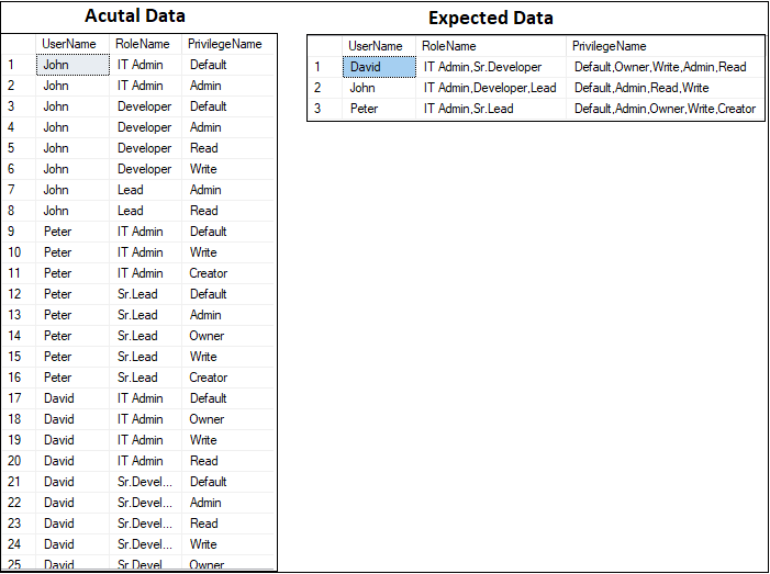
Our user belongs to several roles, each of which has a number of privileges associated with it. The responsibilities and privileges that are linked to each user are what users want to see. In order to prevent redundant roles and privileges, the final product should have distinct roles and privileges. Basically, we have to remove duplicates from the string separated by commas.

Let's look at the data—both real and predicted.
Solution
One of two methods can be used to solve this problem in SQL Server utilizing the STRING_AGG() function.

Method 1
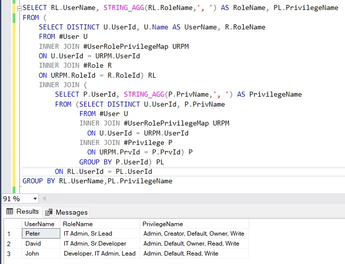
We may efficiently eliminate any duplicates by utilizing STRING_AGG() inside a subquery.

SELECT RL.UserName, STRING_AGG(RL.RoleName,', ') AS RoleName, PL.PrivilegeName
FROM (
    SELECT DISTINCT U.UserId, U.Name AS UserName, R.RoleName
    FROM #User U
    INNER JOIN #UserRolePrivilegeMap URPM
    ON U.UserId = URPM.UserId
    INNER JOIN #Role R
    ON URPM.RoleId = R.RoleId) RL
    INNER JOIN (
        SELECT P.UserId, STRING_AGG(P.PrivName,', ') AS PrivilegeName
        FROM (SELECT DISTINCT U.UserId, P.PrivName
              FROM #User U
              INNER JOIN #UserRolePrivilegeMap URPM
                ON U.UserId = URPM.UserId
              INNER JOIN #Privilege P
                ON URPM.PrvId = P.PrvId) P
              GROUP BY P.UserId) PL
        ON RL.UserId = PL.UserId
GROUP BY RL.UserName,PL.PrivilegeName

Expected Result
Method 2
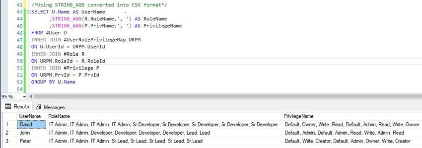
Rows can be converted to Comma-Separated Values (CSV) by utilizing the grouped concatenation method with STRING_AGG(). Then, we can use the XQuery function distinct-values() to retrieve unique values from the XML instance after converting the CSV file to XML.

/*Using XQuery-function distinct-values() get only distinct values*/
SELECT UserName
     ,STUFF((RoleName.query('for $x in distinct-values(/x/text())return <x>{concat(",", $x)}</x>').value('.','varchar(250)')),1,1,'') AS RoleName
     ,STUFF((PrivilegeName.query('for $x in distinct-values(/x/text())return <x>{concat(",", $x)}</x>').value('.','varchar(250)')),1,1,'') AS PrivilegeName
FROM(
SELECT U.Name As UserName
    ,CAST('<x>' + REPLACE(STRING_AGG(R.RoleName,','),',','</x><x>') + '</x>' AS XML) AS   RoleName
    ,CAST('<x>' + REPLACE(STRING_AGG(P.PrivName,','),',','</x><x>') + '</x>' AS XML) AS   PrivilegeName
FROM #User U
INNER JOIN #UserRolePrivilegeMap URPM
ON U.UserId = URPM.UserId
INNER JOIN #Role R
ON URPM.RoleId = R.RoleId
INNER JOIN #Privilege P
ON URPM.PrvId = P.PrvId
GROUP BY U.Name)A

Step 1: Transform the real data into the CSV format indicated below by using the STRING_AGG() function.
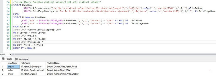
Step 2. Next, convert the CSV into XML format.

Step 3. Now, utilize the XQuery function distinct-values() to extract unique values from the XML instance.
Tables and Insert Scripts
/*Create USER Table and Insert Data*/
DROP TABLE IF EXISTS #User
CREATE TABLE #User (UserId INT, Name VARCHAR(50))
INSERT INTO #User (UserId, Name)
VALUES (1, 'John'),
     (2, 'Peter'),
     (3, 'David')

/*Create ROLE Table and Insert Data*/
DROP TABLE IF EXISTS #Role
CREATE TABLE #Role (RoleId INT, RoleName VARCHAR(50))
INSERT INTO #Role (RoleId, RoleName)
VALUES (1, 'IT Admin'), (2, 'Developer'), (3, 'Sr.Developer'), (4, 'Lead'), (5, 'Sr.Lead')

/*Create PRIVILEGE Table and Insert Data*/
DROP TABLE IF EXISTS #Privilege
CREATE TABLE #Privilege (PrvId INT, PrivName VARCHAR(50))
INSERT INTO #Privilege (PrvId, PrivName)
VALUES (1, 'Default'), (2, 'Admin'), (3, 'Creator'), (4, 'Read'), (5, 'Write'), (6, 'Owner')

/*Create USERROLEPRIVILEGEMAP Table and Insert Data*/
DROP TABLE IF EXISTS #UserRolePrivilegeMap
CREATE TABLE #UserRolePrivilegeMap(UserId INT, RoleId INT, PrvId INT)
INSERT INTO #UserRolePrivilegeMap (UserId, RoleId, PrvId)
VALUES (1,1,1), (1,1,2), (1,2,1), (1,2,2), (1,2,4), (1,2,5), (1,4,2),
     (1,4,4), (2,1,1), (2,1,5), (2,1,3), (2,5,1), (2,5,2), (2,5,6),
     (2,5,5), (2,5,3), (3,1,1), (3,1,6), (3,1,5), (3,1,4), (3,3,1),
     (3,3,2), (3,3,4), (3,3,5), (3,3,6)

/*Join all tables and get the actual data*/
SELECT U.Name AS UserName
    ,R.RoleName
    ,P.PrivName AS PrivilegeName
FROM #User U
INNER JOIN #UserRolePrivilegeMap URPM
ON U.UserId = URPM.UserId
INNER JOIN #Role R
ON URPM.RoleId = R.RoleId
INNER JOIN #Privilege P
ON URPM.PrvId = P.PrvId

Conclusion
Efficiently convert row data into comma-separated values using SQL Server's string aggregate function, ensuring duplicates are removed for streamlined data representation and integrity.

HostForLIFEASP.NET SQL Server 2022 Hosting


European SQL Server 2022 Hosting :: Setting Up a Calendar in SQL Server

clock May 3, 2024 08:20 by author Peter

Using SQL Server's built-in capabilities, I've made a basic calendar in the example below.

Temporary SQL Server Tables
The instantaneous result sets that are queried repeatedly can be stored in the temporary tables.

Setting up makeshift tables

SELECT INTO and CREATE TABLE statements are the two methods that SQL Server offers for creating temporary tables.

CREATE OR ALTER PROCEDURE calender(@start_date DATE, @end_date DATE)
AS
BEGIN
    DECLARE @DateDiff INT;
    DECLARE @count INT;
    SET @count = 0; -- DAY ONE COUNT OF START DATE
    SET @DateDiff = DATEDIFF(DAY, @start_date, @end_date); -- DIFF BTW TWO DATE
    DROP TABLE IF EXISTS #temp_cal;
    CREATE TABLE #temp_cal(
        id INT IDENTITY(1,1) PRIMARY KEY,
        d_date DATE,
        end_date DATE
    );
    WHILE @count <= @DateDiff BEGIN
        INSERT INTO #temp_cal(d_date, end_date) VALUES(DATEADD(DAY, @count, @start_date), @end_date);
        SET @count = @count + 1;
    END;
    SELECT DAY(d_date) AS 'DAY',
           MONTH(d_date) AS 'MONTH',
           DATENAME(weekday, d_date) AS 'DAY_NAME',
           DATENAME(month, d_date) AS 'MONTH_NAME',
           DATENAME(year, d_date) AS 'YEAR',
           d_date AS 'DATE',
           DATENAME(week, d_date) AS 'WEEK',
           DATEPART(DY, d_date) AS 'DAY_OF_YEAR',
           DATEPART(ISO_WEEK, d_date) AS 'ISO_WEEK',
           DATEPART(wk, d_date) AS 'US WEEK',
           DATEPART(wk, d_date) AS 'WEEK_OF_YEAR',
           DATEDIFF(DAY,d_date, end_date) AS 'NUMBER_OF_DAYS_IN_MONTH',
           DATEDIFF(WEEK,d_date,end_date) AS 'WEEKS_IN_YEAR',
           DATEDIFF(MONTH,d_date,end_date) AS 'MONTHS_IN_YEAR',
           FORMAT(d_date, 'D', 'en-US' ) AS 'CULTURES_FOR_US'
    FROM #temp_cal;
END;
EXEC calender @start_date = '2023-01-01', @end_date = '2023-12-31';

HostForLIFEASP.NET SQL Server 2022 Hosting


About HostForLIFE

HostForLIFE is European Windows Hosting Provider which focuses on Windows Platform only. We deliver on-demand hosting solutions including Shared hosting, Reseller Hosting, Cloud Hosting, Dedicated Servers, and IT as a Service for companies of all sizes.

We have offered the latest Windows 2019 Hosting, ASP.NET 5 Hosting, ASP.NET MVC 6 Hosting and SQL 2019 Hosting.


Month List

Tag cloud

Sign in